Learn SQL with Datasette

This tutorial follows the tutorial on exploring data with Datasette and shows how you can use Datasette to start learning to write custom SQL queries of your own.

We will be using the same example database as that tutorial:

https://congress-legislators.datasettes.com/legislators

This database contains information about US Presidents, Vice Presidents and Members of Congress from 1789 to today. You can follow the previous tutorial to become familiar with the data.

SQL and SQLite

Datasette is software that runs on top of a SQL database. There are many different SQL database systems, such as MySQL, PostgreSQL, Microsoft SQL Server and Oracle. The database used by Datasette is called SQLite.

You may not realize it, but you already use SQLite every day: it is built into many popular applications, including Google Chrome and Firefox, and runs on laptops, iPhones, Android phones and all sorts of other smaller devices.

SQL stands for Structured Query Language - it is a text language for running queries against a database. Every database implements a slightly different dialect of SQL - for this tutorial I will try to keep to the subset of SQLite's dialect that is most likely to work across other databases as well.

View and edit SQL

Every table page in Datasette - such as this one - includes a "View and edit SQL" link that looks like this:

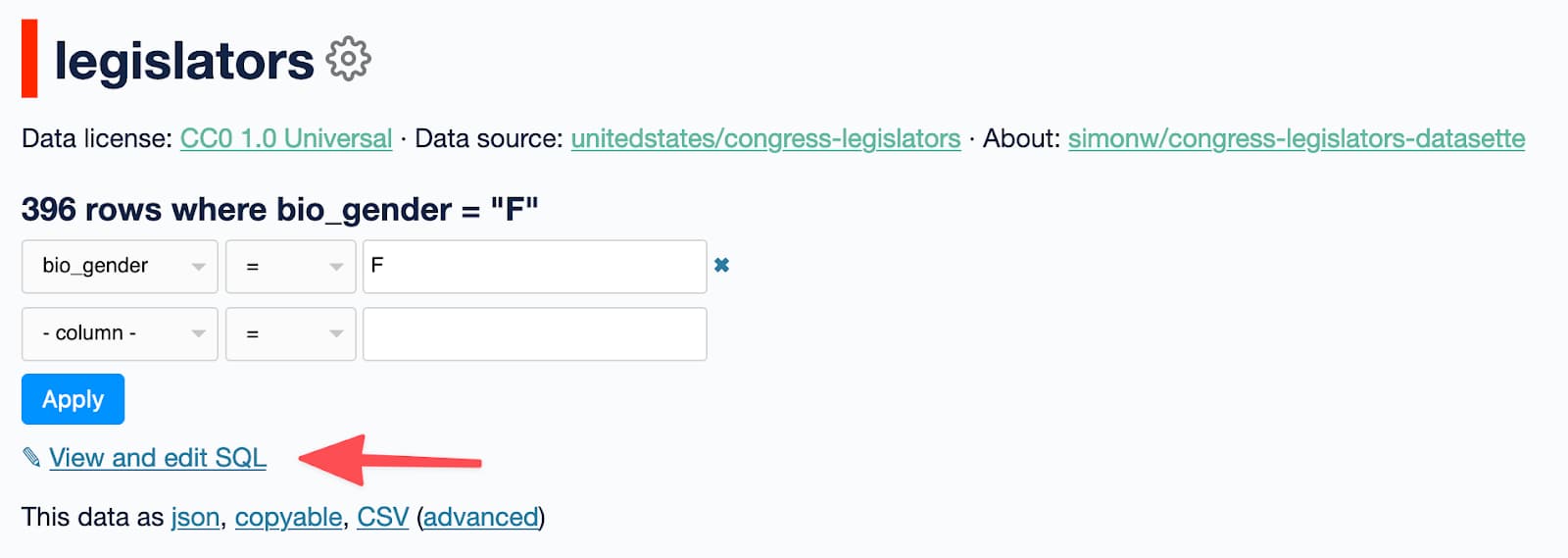
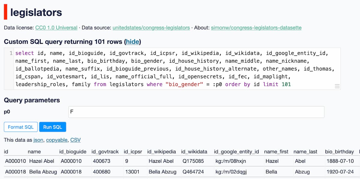
Click that link to see the SQL query that was used for the current page - including any filters that have been applied, in this case the filter for bio_gender = 'F'.

You can then edit that query to make it do something else!

Exercises

Start with that example, then:

1. Click "Format SQL" to tidy this up and make it easier to read and edit
2. Modify that query to return only the id and name columns
3. Get it to order by name instead of sorting by id
4. Change the p0 value to M to return male instead of female legislators
5. Try replacing the list of columns with select * from - a shortcut for all columns

The structure of a basic select query

Here's the formatted version of the above query:

select
  id,
  name,
  id_bioguide,
  id_govtrack,
  id_icpsr,
  id_wikipedia,
  id_wikidata,
  id_google_entity_id,
  name_first,
  name_last,
  bio_birthday,
  bio_gender,
  id_house_history,
  name_middle,
  name_nickname,
  id_ballotpedia,
  name_suffix,
  id_bioguide_previous,
  id_house_history_alternate,
  other_names,
  id_thomas,
  id_cspan,
  id_votesmart,
  id_lis,
  name_official_full,
  id_opensecrets,
  id_fec,
  id_maplight,
  leadership_roles,
  family
from
  legislators
where
  bio_gender = :p0
order by
  id
limit
  101

select

The select section specifies which columns you would like to return. Each column name is separated by a comma - but if you have a comma following the last column you you will get an error message.

near from: syntax error

from

The from section specifies which table the records should be selected from - here we want the legislators table.

where

The where section adds filter conditions. These can be combined using and, for example this query will select just legislators who are male and have a Jr. name suffix:

where
  bio_gender = 'M'
  and name_suffix = 'Jr.'

This section is optional - if you do not include a where clause you will get back every row in the table.

order by

The optional order by clause specifies the order you woud like the rows to be returned in. This would order them alphabetically by name:

order by
  name

Or add desc to reverse the order. This query returns the youngest legislators:

select
  *
from
  legislators
order by
  bio_birthday desc

limit

The limit 101 clause limits the query to returning just the first 101 results. In most SQL databases omitting this will cause all results will be returned - but Datasette applies an additional limit of 1,000 (example here) to prevent large queries from causing performance issues.

Named parameters

In the previous tutorial we used filters to list presidental terms that occurred in the 1800s, by filtering on rows where the start column began with the string 18 and the type column equals prez.

Here's that example as a filtered table.

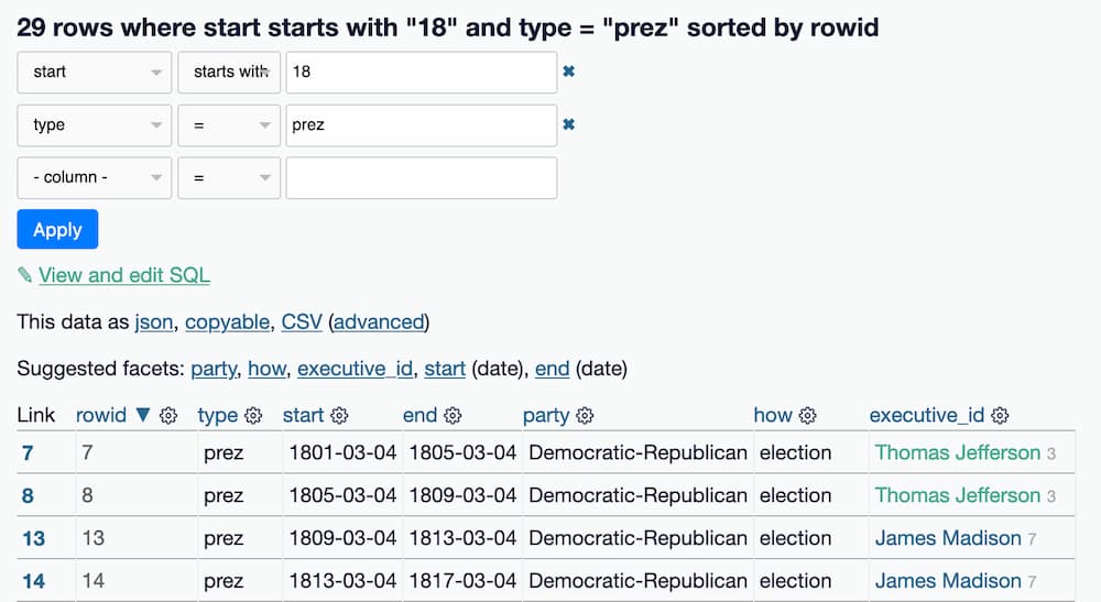
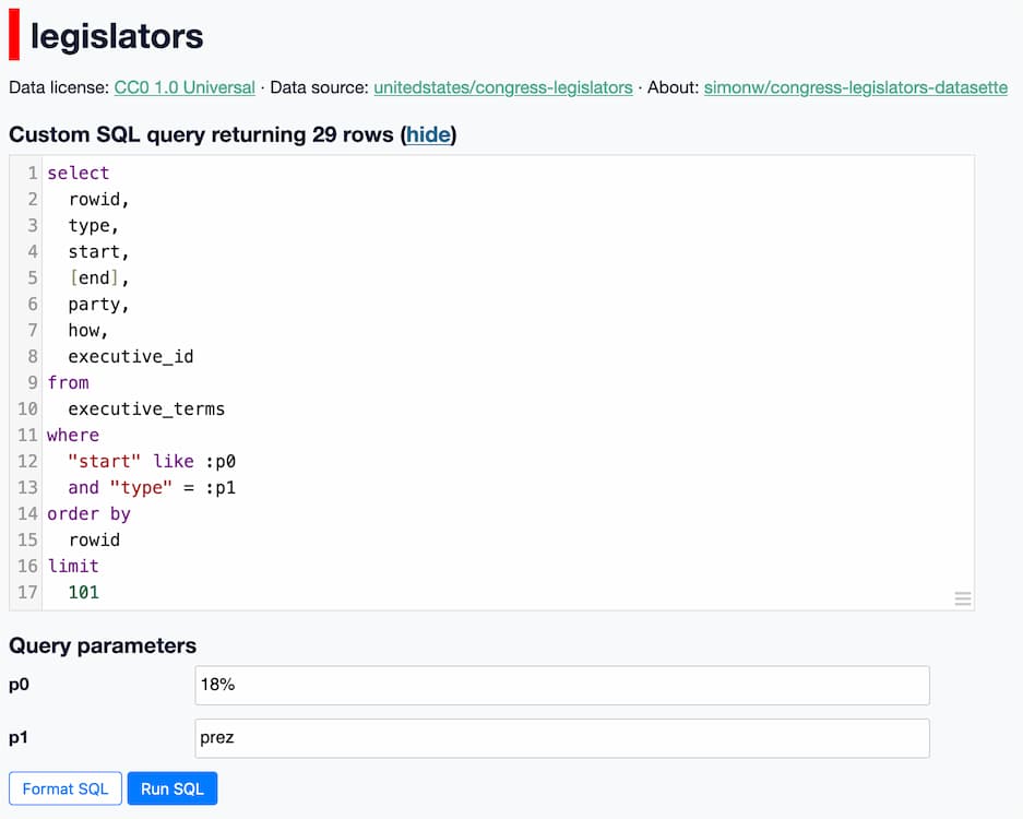
Clicking that "View and edit SQL" link (and then clicking "Format SQL") shows this query:

select
  rowid,
  type,
  start,
  end,
  party,
  how,
  executive_id
from
  executive_terms
where
  start like :p0
  and type= :p1

The :p0 and :p1 fields here correspond to "named parameters" - they provide a safe way to pass values to a SQL query, without having to worry about SQL injection.

These field names are extracted from the query. If you change the where clause to look like this:

where
  start like :century
  and type = :type

Then fields called century and type will be displayed instead of p0 and p1.

Since they are form fields, you can change those values too. Try changing prez to viceprez to see the vice presidential terms for the 1800s instead.

If you weren't using named parameters, the where clause of the query could look like this instead:

where
  start like '18%'
  and type = 'prez'

String values like '18%' and 'prez' must be enclosed in single or double quotes (single quotes are preferred), if you are not using the :p0 syntax.

The double quotes around the column names here are optional - they are only required if the column has a name that might clash with an existing SQL keyword, such as select or where - or if the column name contains a space. So the following where clause would work the same way:

where
  start like '18%'
  and type = 'prez'

SQL LIKE queries

To find rows where the start column begins with the string 18 we use this where filter:

where
  start like '18%'

The SQL like operator applies wildcards to strings - % means "match anything" and _ (underscore) means "match a single character".

Exercise

• Use a LIKE filter to find presidential terms that occurred in the 90s decade of any century - you'll need to use both _ and % for this. (solution)

SQL Joins

The executive_terms table has a column called executive_id which displays both a numeric ID and a link containing the name of the executive:

But... when you click the "View and edit SQL" link the resulting query returns just the ID, not the name.

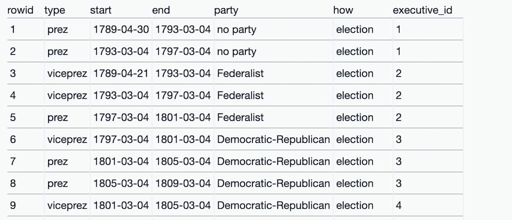
A SQL join can be used to combine the data from multiple tables. Here's a query that uses a join to show the name pulled from the executives table:

select
  executive_terms.type,
  executive_terms.start,
  executive_terms.end,
  executive_terms.party,
  executive_terms.how,
  executives.name
from
  executive_terms
  join executives
    on executive_terms.executive_id = executives.id

Try that here.

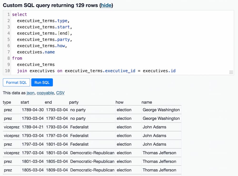
Since there are now two tables involved in the query, it's a good idea to include explicit table names as part of the select clause:

select
  executive_terms.type,
  executive_terms.start,
  executive_terms.end,
  executive_terms.party,
  executive_terms.how,
  executives.name

If a column exists in only one of the two tables you can use its name without specifying the table, but this can quickly get confusing so it's better to always use the table names when you are executing a join.

The from clause is where the join is defined. This describes how the two tables should be combined together:

from
  executive_terms
  join executives
    on executive_terms.executive_id = executives.id

We are joining executive_terms to executives, using the fact that the executive_id column in executive_terms contains values from the id column in executives.

This is why IDs and foreign keys are important concepts to understand in SQL databases!

This kind of join is also known as an "inner join" - it is the most commonly used join. Other join types include outer joins and full joins, but those are beyond the scope of this tutorial.

GROUP BY / COUNT

A common operation in SQL is to ask for a count of the most popular values in a column.

Datasette exposes this capability in its faceting feature. Under the hood, that feature works by executing a group by / count query.

The following query answers the question: which party has had the most presidental terms?

select
  party,
  count(*)
from
  executive_terms
where
  type = 'prez'
group by
  party

Try that query here.

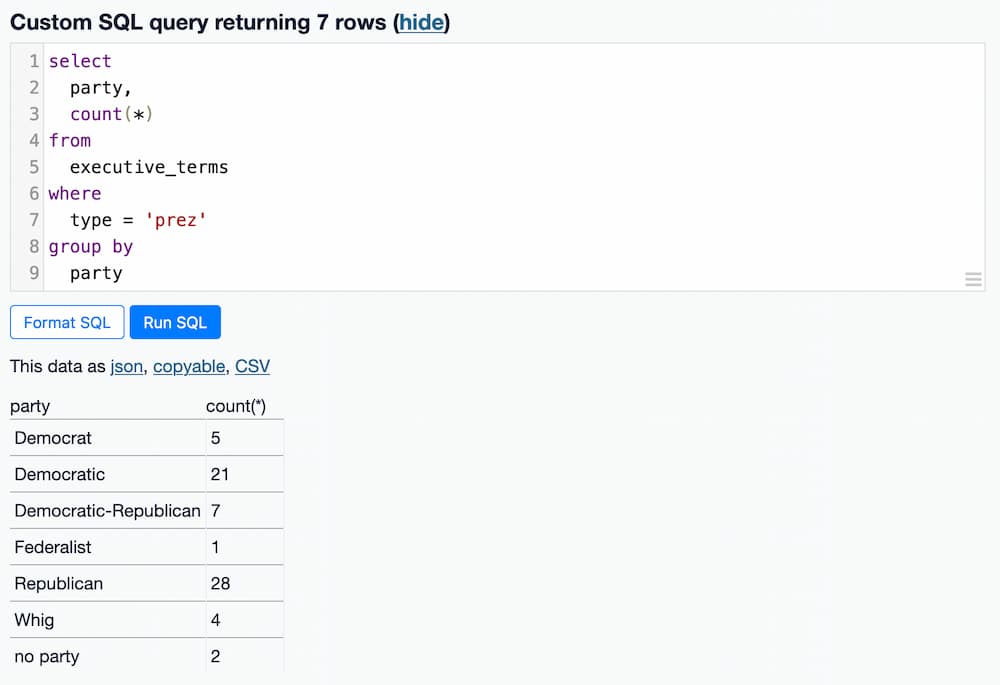
The select clause asks for the party column and the result of running a count(*). count() is a SQL aggregate function, which operates on a group of results. So we need to define a group.

The group by party clause at the end creates those groups. The combination of the two produces the desired result.

You can add this order by clause at the end to see the groups sorted from highest to lowest:

order by
  count(*) desc

Here's the result.

WHERE ... IN

SQL queries can be nested together in a number of interesting ways.

One of the most useful for ad-hoc data analysis is the where column in (select ...) pattern.

Let's build a query to see everyone who has been president and has also been vice president.

We'll start with a query to return the names of every vice president. This requires a join against executives, because the executive_terms table includes the presidential and vice presidential terms, but doesn't include the names of those individuals.

select
  executives.name
from
  executive_terms
  join executives
    on executive_terms.executive_id = executives.id
where
  type = 'viceprez'

This query returns 61 rows, including some duplicate rows for individuals who served more than one term as VP.

We could use select distinct to remove those duplicates if we wanted to.

If we want to see everyone who has been a president and ALSO been a vice-president, we can combine two queries together like this:

select
  distinct executives.name
from
  executive_terms
  join executives
    on executive_terms.executive_id = executives.id
where
  type = 'prez'
  and name in (
    select
      executives.name
    from
      executive_terms
      join executives
        on executive_terms.executive_id = executives.id
    where
      type = 'viceprez'
  )

This query returns 15 names, starting with John Adams and finishing with Joseph Biden.

⚠️ An earlier version of this example revealed a subtle bug: there were two separate individuals in the executives table with the same name, George Bush and George Bush! So even though the query appeared to return the correct results it actually contained a bug. This is a useful demonstration of how important it is to work with unique, de-duplicated identifiers where-ever possible, rather than assuming that things like names are unique.

Common Table Expressions

This is a more advanced SQL technique that I find myself using every day: it can make complex SQL queries much easier to write and understand.

Common Table Expressions, or CTEs, allow you to define a temporary alias for a select that lasts for the duration of the current query. You can then treat it as if it was a regular table.

Here's an example that creates two CTEs, one called presidents and one called vice_presidents, and then uses them to answer the earlier question about presidents who had also served as vice presidents:

with presidents as (
  select
    executives.name
  from
    executive_terms
    join executives
      on executive_terms.executive_id = executives.id
  where
    executive_terms.type = 'prez'
),
vice_presidents as (
  select
    executives.name
  from
    executive_terms
    join executives
      on executive_terms.executive_id = executives.id
  where
    executive_terms.type = 'viceprez'
)
select
  distinct name
from
  presidents
where name in vice_presidents

Try this CTE query here.

The two CTEs are defined using with alias_name as (select ...), second_alias as (select ...) - then the query that returns the final results is added on at the end.

Creating bookmarkable apps

Since every page on Datasette can be linked to (see Sharing links) and named parameters automatically add form input to the query page, you can combine these two features to create bookmarkable apps.

This is particularly useful for collaborating with others who don't yet know SQL. You can write SQL queries that solve problems for them, add parameters that they can customize and then send them the entire custom application as a link that they can bookmark.

Let's create an application that returns the president and vice president for any given date.

Here's the SQL query we will be using:

select
  executives.name,
  executive_terms.type,
  executive_terms.start,
  executive_terms.end,
  executive_terms.party
from
  executive_terms
  join executives
    on executive_terms.executive_id = executives.id
where
  start <= :date
  and end > :date

This query takes a :date parameter, which should be of the format yyyy-mm-dd - for example 2016-01-01.

It joins against the executives table to get their name, and then filters to rows where the term start is less than or equal to the specified date, and the end is greater than that date. We use <= for one of these to ensure there are no gaps or overlaps.

If we execute the query without a date it will return 0 results, but give us a form field to enter the date:

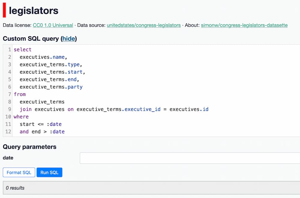
Entering a date - for example 2016-01-01 - returns the president and vice president for that date:

We've built an application! We can send this link to anyone right now and they'll be able to run that same query.

The SQL at the top of the page could feel a little intimidating though. That's what the "hide" link is for - clicking on that hides the SQL query, providing a new link that you can share that won't cause the user to scroll down past the SQL in order to interact with the query.

One last note: the application we have built also doubles up as an API. Add .json to the path portion of the URL, or click the .json link, to get back the data as JSON. Add &_shape=array to the URL to get back a more compact form of JSON, ideal for integrating with other applications.

Next steps

Fully mastering SQL can take years. This tutorial has attempted to cover SQL basics and introduce some more advanced techniques to help manage larger queries, but there's plenty more to learn. The SQLite SELECT documentation offers a comprehensive reference to SQL as understood by SQLite, but the best way to learn is to keep on trying new things against different data, looking things up as you go along.